Excel Highlight Row

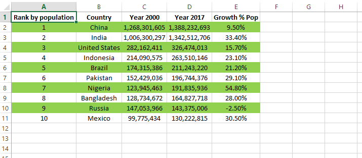
When your table is huge, it is easier to read the data when every other row are filled with different colors. In this example, we will demonstrate how to fill colors alternately. This trick can also highlight every third row in Excel (4th row, 5th row and so on).

How is it done
Step 1. Select the Excel data.

Step 2. Go to Home > Conditional Formatting > New Rule > Use a formula to determine which cells to format. See screenshot below for details.

Step 3. Type in the formula =mod(row(),2)=0 (as shown below). Then press 'Format..', new small window will pop out, click 'Fill' tab. Select the desired color (in this example we chose green), press 'OK'.

There is another way to fill colors in sequence, this can be done using our multi-tool add-in. The colors set by this add-in are applied to the cells directly (not through conditional formatting), this means the color will stay when you delete row/rows.